R

Reading the regions in R, and assigning regions to data

The measoshapes package

remotes::install_github("AustralianAntarcticDivision/measoshapes")
library(measoshapes)

The package has the regions as sf data sets, one row per region (20 rows), with columns name, label, sector, zone and fill:

measo_regions06, measo_regions06_coastline: polar equal area
measo_regions06_ll, measo_regions06_ll_coastline: longitude/latitude
measo_names06: the columns alone

measo_regions06

Simple feature collection with 20 features and 5 fields
Geometry type: POLYGON
Dimension:     XY
Bounding box:  xmin: -6381686 ymin: -6381694 xmax: 6381694 ymax: 6381694
Projected CRS: +proj=laea +lat_0=-90 +lon_0=0 +x_0=0 +y_0=0 +datum=WGS84 +units=m +no_defs
   name                       label        sector         zone    fill
1   AOA          Antarctic Atlantic      Atlantic    Antarctic #F9BDBC
2   AOS       Subantarctic Atlantic      Atlantic Subantarctic #F27071
3   AON           Northern Atlantic      Atlantic     Northern #E11F26
4   AOT          Temperate Atlantic      Atlantic         <NA>    <NA>
5   CIA    Antarctic Central Indian CentralIndian    Antarctic #F9D7C2
6   CIS Subantarctic Central Indian CentralIndian Subantarctic #F4B187
7   CIN     Northern Central Indian CentralIndian     Northern #EC8444
8   CIT    Temperate Central Indian CentralIndian         <NA>    <NA>
9   EIA       Antarctic East Indian    EastIndian    Antarctic #D1D3EA
10  EIS    Subantarctic East Indian    EastIndian Subantarctic #B0B4D9
11  EIN        Northern East Indian    EastIndian     Northern #878DC5
12  EIT       Temperate East Indian    EastIndian         <NA>    <NA>
13  WPA      Antarctic West Pacific   WestPacific    Antarctic #E0B8D6
14  WPS   Subantarctic West Pacific   WestPacific Subantarctic #C579B2
15  WPN       Northern West Pacific   WestPacific     Northern #843A75
16  WPT      Temperate West Pacific   WestPacific         <NA>    <NA>
17  EPA      Antarctic East Pacific   EastPacific    Antarctic #9FC5C7
18  EPS   Subantarctic East Pacific   EastPacific Subantarctic #609FA0
19  EPN       Northern East Pacific   EastPacific     Northern #4B7E7F
20  EPT      Temperate East Pacific   EastPacific         <NA>    <NA>
                         geometry
1  POLYGON ((-2891647 1737477,...
2  POLYGON ((1842392 3191116, ...
3  POLYGON ((2613013 4525871, ...
4  POLYGON ((-3353009 1723416,...
5  POLYGON ((279139.2 483483.3...
6  POLYGON ((1842392 3191116, ...
7  POLYGON ((2294977 3975017, ...
8  POLYGON ((2613013 4525871, ...
9  POLYGON ((3048452 -1421517,...
10 POLYGON ((533521.3 -3025749...
11 POLYGON ((4093993 -1909060,...
12 POLYGON ((4882884 -2276926,...
13 POLYGON ((524717.5 -3027289...
14 POLYGON ((9312.405 -2801188...
15 POLYGON ((637964.6 -3618077...
16 POLYGON ((16836.49 -4961088...
17 POLYGON ((-457314.9 -320215...
18 POLYGON ((-2250033 -1575490...
19 POLYGON ((-2992183 -2095149...
20 POLYGON ((-4421564 -3096013...

Version 05 is in the package as released (measo_regions05 etc., 24 rows with the West Pacific regions in two pieces, and measo_names row-aligned with them); see the README.

The files on the Data page (one row per region) are in the package too:

f <- system.file("extdata/measo_regions06.parquet", package = "measoshapes")

Reading from a URL

No package installation is needed to read the published files. GDAL reads them directly from the URL.

u <- "https://australianantarcticdivision.github.io/measoshapes/data/v06/measo_regions06.parquet"

## sf
x <- sf::read_sf(u)

## terra
v <- terra::vect(u)

## gdalraster
lyr <- gdalraster::GDALVector$new(paste0("/vsicurl/", u))
d <- lyr$fetch(-1)
lyr$close()

## arrow, geometry as well-known binary (wk/geoarrow)
library(geoarrow)
tab <- arrow::read_parquet(u)

FlatGeobuf and GeoJSON work the same way (change the file name), and are a good choice if your GDAL doesn’t have the Parquet driver (check "Parquet" %in% sf::st_drivers()$name).

Assigning regions to data

To find the region for longitude/latitude locations, transform them to the polar equal area projection and join with the polar regions:

regions <- read_sf(file.path(dd, "measo_regions06.parquet"))  ## or the URL above
pts <- data.frame(lon = c(147.3, 100.5, -10.5, -82.5, 171.5, -175.5),
                  lat = c(-50.2, -60.5, -70.5, -45.5, -65.5, -65.5))
p <- st_as_sf(pts, coords = c("lon", "lat"), crs = "OGC:CRS84", remove = FALSE)
p <- st_join(st_transform(p, st_crs(regions)), regions)
st_drop_geometry(p)

     lon   lat name                    label        sector      zone    fill
1  147.3 -50.2  EIN     Northern East Indian    EastIndian  Northern #878DC5
2  100.5 -60.5  CIA Antarctic Central Indian CentralIndian Antarctic #F9D7C2
3  -10.5 -70.5  AOA       Antarctic Atlantic      Atlantic Antarctic #F9BDBC
4  -82.5 -45.5  EPN    Northern East Pacific   EastPacific  Northern #4B7E7F
5  171.5 -65.5  WPA   Antarctic West Pacific   WestPacific Antarctic #E0B8D6
6 -175.5 -65.5  WPA   Antarctic West Pacific   WestPacific Antarctic #E0B8D6

The polar regions are densified to 0.2° from the longitude/latitude definition, so this agrees with the definition except for locations within a very short distance of a boundary.

For gridded data, the same applies: classify cell centres, or rasterize the polar regions onto your grid (e.g. terra::rasterize(terra::vect(regions), grid, field = "name")).

Maps

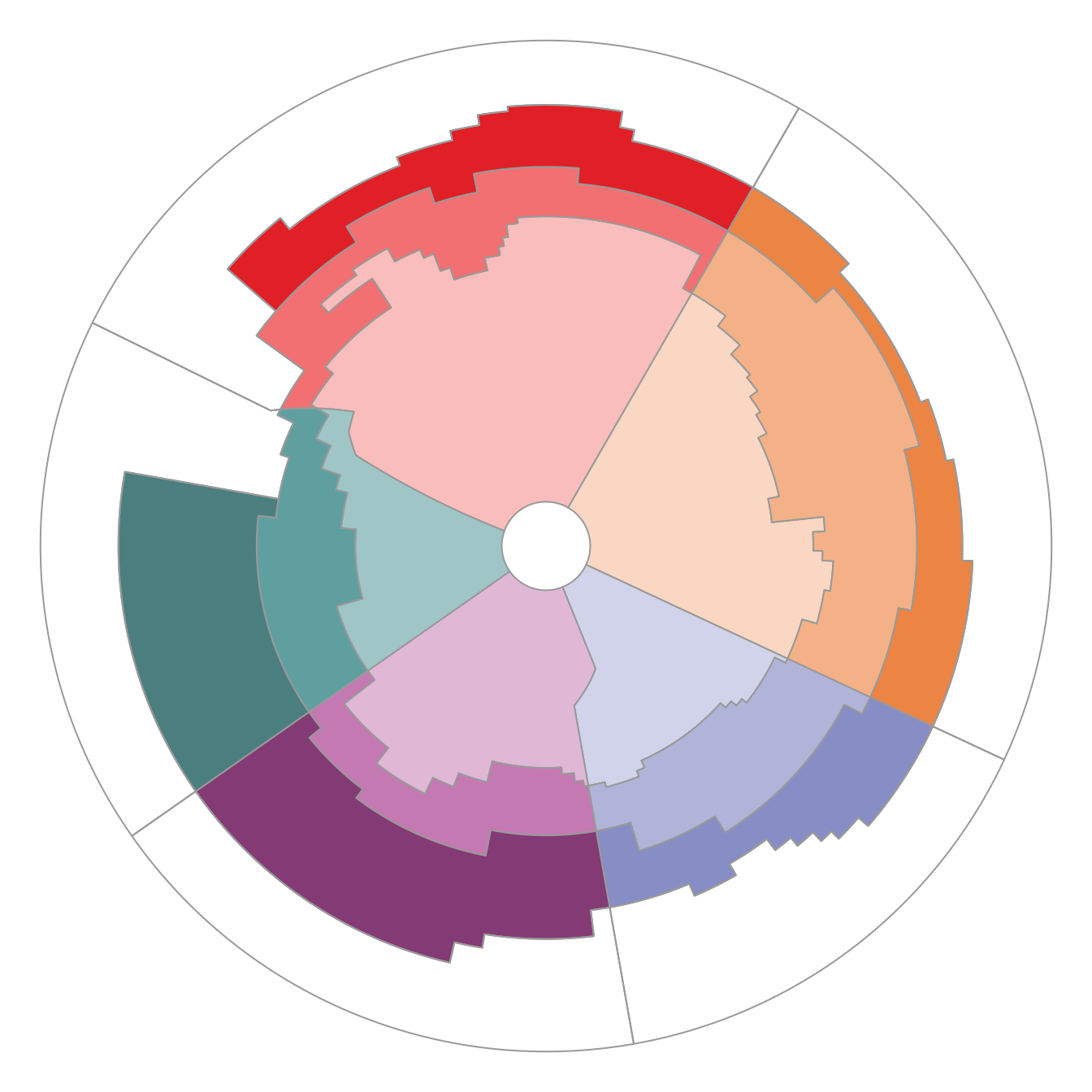
par(mar = rep(0, 4))
plot(st_geometry(regions), col = regions$fill, border = "grey60")

Figure 1: Base graphics with the fill colours.

With ggplot2, use the colours as they are with scale_fill_identity():

library(ggplot2)
ggplot(regions, aes(fill = fill)) + geom_sf(colour = "grey60") + scale_fill_identity()