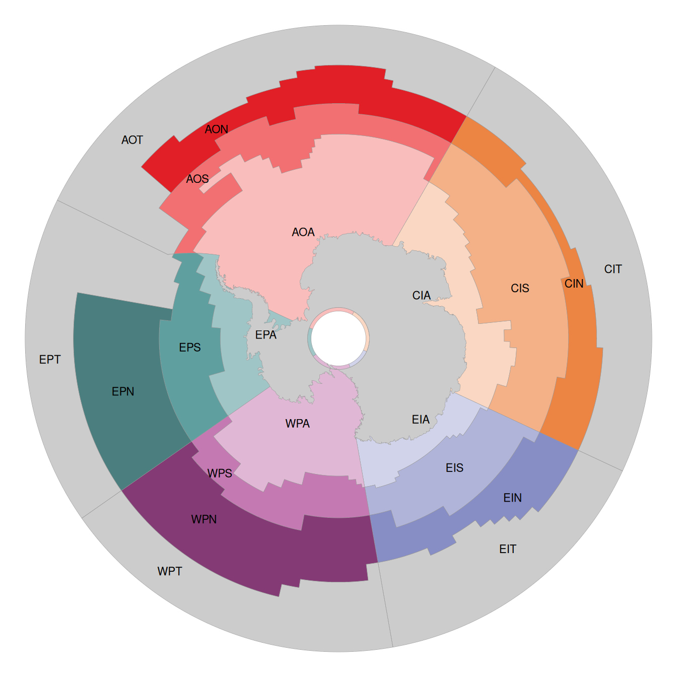
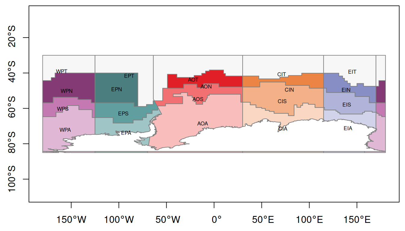
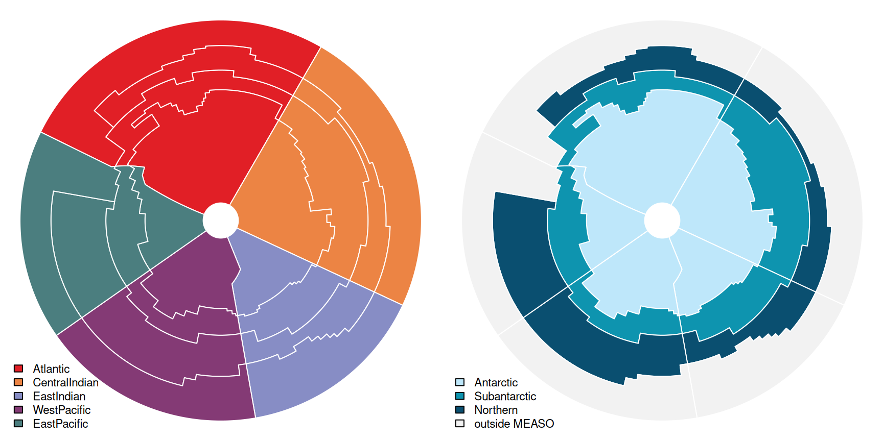
All figures on this page are made in R from the published files and the package data sets; expand “Code” to see how.
Colours
The colours of the MEASO Summary for Policymakers (Figure 5); see Definition .
Code
<- function (x) {<- function (name, fill) {if (is.na (fill)) return (sprintf ("<td>%s</td>" , name))<- col2rgb (fill)<- if (sum (rgb * c (0.299 , 0.587 , 0.114 )) > 140 ) "black" else "white" sprintf ('<td style="background:%s;color:%s">%s<br><code style="background:none;color:%s">%s</code></td>' ,substr (fill, 1 , 7 ), fg, name, fg, substr (fill, 1 , 7 ))<- c ("Antarctic" , "Subantarctic" , "Northern" , NA )<- vapply (unique (x$ sector), function (s) {<- x[x$ sector == s, ]<- vapply (zones, function (z) {<- which (if (is.na (z)) is.na (d$ zone) else d$ zone %in% z)cell (d$ name[i], d$ fill[i])"" )sprintf ("<tr><th>%s</th>%s</tr>" , s, paste (cells, collapse = "" ))"" )cat ('<table class="table" style="text-align:center">' ,"<tr><th></th><th>Antarctic</th><th>Subantarctic</th><th>Northern</th><th>(outside)</th></tr>" ,"</table>" , sep = " \n " )colour_table (x)
Version 05 colours
The colours of version 05 (measo_names in the R package), as released. Sectors that alternate around the continent share a palette. The first of the two West Pacific Antarctic (WPA) rows in measo_names has a different colour (an error); this table shows the second.
Code
colour_table (measo_names[! duplicated (measo_names$ name, fromLast = TRUE ), ])
Polar map
Code
<- measo_regions06_coastlinepar (mar = rep (0 , 4 ))plot (st_union (st_geometry (x)), col = "grey80" , border = NA ) ## continent shows through plot (st_geometry (cst), col = cst$ fill, border = "grey60" , lwd = 0.3 , add = TRUE )<- st_coordinates (suppressWarnings (st_point_on_surface (st_geometry (x))))text (pos, x$ name, cex = 0.7 )
Longitude/latitude map
Code
<- measo_regions06_ll_coastlinepar (mar = c (2.5 , 2.5 , 0.5 , 0.5 ))plot (st_geometry (ll), col = ifelse (is.na (ll$ fill), "grey97" , ll$ fill),border = "grey50" , axes = TRUE , xlim = c (- 180 , 180 ), ylim = c (- 85 , - 30 ))## label positions from the polar centroids <- st_coordinates (st_transform (st_centroid (st_geometry (measo_regions06)), 4326 ))text (cds, measo_regions06$ name, cex = 0.55 )
Sectors and zones
Code
<- par (mfrow = c (1 , 2 ), mar = rep (0.2 , 4 ))## each sector's hue (its Northern zone colour) <- with (x[x$ zone %in% "Northern" , ], setNames (fill, sector))plot (st_geometry (x), col = sec_col[x$ sector], border = "white" )legend ("bottomleft" , legend = names (sec_col), fill = sec_col, bty = "n" , cex = 0.7 )<- c (Antarctic = "#BEE7FA" , Subantarctic = "#0E94AF" , Northern = "#0A4F70" )plot (st_geometry (x), col = ifelse (is.na (x$ zone), "grey95" , zone_col[x$ zone]), border = "white" )legend ("bottomleft" , legend = c (names (zone_col), "outside MEASO" ), fill = c (zone_col, "grey95" ),bty = "n" , cex = 0.7 )par (op)
Areas
Areas are calculated in the polar equal area projection, for the full regions and with the continent cut out.
Code
<- data.frame (name = measo_regions06$ name, label = measo_regions06$ label,full = round (as.numeric (st_area (measo_regions06)) / 1e12 , 2 ),without_continent = round (as.numeric (st_area (measo_regions06_coastline)) / 1e12 , 2 )):: kable (tab, row.names = FALSE )
Plots on a map
The regions make a natural layout for small plots of data summarised by region. The map-patches vignette in the R package shows one way to do this with ggplot2 and patchwork.