Definition

What the regions are, how they are built, and why

Note

This page describes version 06. Its boundaries are those of version 05, built by data-raw/munge-sectors05.R; version 06 is made from version 05 by data-raw/munge-sectors06.R (see History).

Sectors and zones

Each region is a combination of a sector and a zone. These are the MEASO assessment areas of the MEASO Summary for Policymakers (Constable et al. 2023, Figure 5), adapted from McCormack et al. (2021); see References.

  • Sectors (west to east from the Pacific): West Pacific, East Pacific, Atlantic, Central Indian, East Indian. Their boundaries are near 125°W, the Drake Passage and Antarctic Peninsula, 30°E, 115°E, and 158–170°E (with a dog-leg at the Ross Sea).
  • Zones (south to north): Antarctic (south of the Southern Antarctic Circumpolar Current Front, SACCF), Subantarctic (SACCF to the Subantarctic Front, SAF), Northern (SAF to the Subtropical Front, STF).
  • North of the STF, to 30°S, each sector has a T region (temperate). These are not part of MEASO; they have no zone and no colour, and exist so that every location in the domain falls in exactly one region.

Region names are the sector code followed by the zone code, e.g. EIS is East Indian Subantarctic.

Sector Code Antarctic Subantarctic Northern (outside)
West Pacific WP WPA WPS WPN WPT
East Pacific EP EPA EPS EPN EPT
Atlantic AO AOA AOS AON AOT
Central Indian CI CIA CIS CIN CIT
East Indian EI EIA EIS EIN EIT

Construction

The regions are not drawn as polygons. They are built from lines:

  1. sector boundary lines, extended from 85°S to 30°S,
  2. the three fronts, as simplified, stair-stepped lines around the whole Southern Ocean,
  3. the edges of the domain: 85°S, 30°S, and the anti-meridian.

The lines are noded together and polygonized (sf::st_polygonize()), very small slivers are dropped, and the polygons are named. Because every polygon comes from the same set of lines, the regions share their boundaries exactly: there are no gaps or overlaps, and together they cover the domain.

Code
## sector lines, as in data-raw/munge-sectors05.R
minlat <- -85; maxlat <- -30
s <- data.frame(lon = c(-125, -125,  -70, -64.5, -60, -55.054477039271191, -63.799776827053591, -63.799776827053591,
                        30, 30,   115, 115,   158, 158, 170, 170, 170),
                lat = c(minlat, maxlat,  minlat, -66, -64, -63.260598133971456, -54.721070105901589, maxlat,
                        minlat, maxlat,   minlat, maxlat,   minlat, -75, -71.60, -47.50, maxlat),
                id = c(1, 1, rep(2, 6), 3, 3, 4, 4, rep(5, 5)))
sectors <- st_sfc(lapply(split(s, s$id), \(d) st_linestring(cbind(d$lon, d$lat))))
load("../data-raw/zones.Rdata")
fronts <- st_geometry(zones)
domain <- st_sfc(st_linestring(cbind(c(-180, 180, 180, -180, -180), c(minlat, minlat, maxlat, maxlat, minlat))))

op <- par(mfrow = c(4, 1), mar = c(0.5, 0.5, 1.5, 0.5))
lim <- list(xlim = c(-180, 180), ylim = c(minlat, maxlat))
plot(domain, col = "grey80", xlim = lim$xlim, ylim = lim$ylim, main = "(a) sectors")
plot(sectors, add = TRUE, lwd = 2)
plot(domain, col = "grey80", main = "(b) fronts")
fcol <- c("#1b9e77", "#d95f02", "#7570b3")
plot(fronts, add = TRUE, lwd = 2, col = fcol)
legend("bottomleft", legend = c("SACCF", "SAF", "STF"), col = fcol, lwd = 2, bty = "n", horiz = TRUE)
plot(domain, lwd = 2, main = "(c) all lines")
plot(sectors, add = TRUE); plot(fronts, add = TRUE)
ll <- st_set_crs(measo_regions06_ll, NA)  ## planar, as in (a)-(c)
plot(st_geometry(ll), col = ifelse(is.na(ll$fill), "grey95", ll$fill),
     border = "grey40", main = "(d) regions")
par(op)
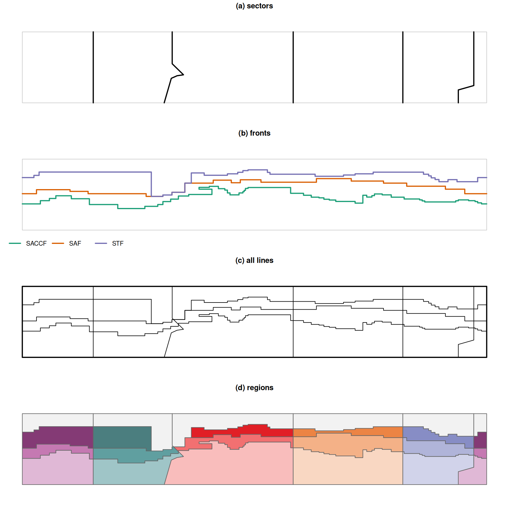
Figure 1: Construction in longitude/latitude: (a) sector lines, (b) fronts (SACCF, SAF, STF), (c) all lines with the domain, (d) the resulting regions.

Boundaries are straight in longitude/latitude

The regions are defined in longitude/latitude as a plane: each boundary segment is a straight line in longitude and latitude. Most segments run along a parallel or a meridian (the fronts are stair-stepped), so “straight in longitude/latitude” means a boundary at 30°S follows the 30°S parallel. This is the same interpretation as GeoJSON (RFC 7946: “a line between two positions is a straight Cartesian line”).

The polar versions are derived from this definition: each boundary is densified to 0.2° in longitude/latitude, then projected to a south polar Lambert Azimuthal Equal Area projection (+proj=laea +lat_0=-90 +lon_0=0 +datum=WGS84, equivalent to EPSG:6932). The polar version can be used directly for areas. The EPSG:3031 (polar stereographic) version is projected from the polar version, for use with Quantarctica and similar.

The anti-meridian

The West Pacific sector crosses the anti-meridian (180°), so in longitude/latitude each West Pacific region is two pieces. In version 06 each region is one row: a single polygon in the polar versions, and a two-part multipolygon in longitude/latitude. (In version 05 the pieces are separate rows: 24 rows, WP names appear twice, and measo_names is row-aligned with them.)

Coastline

The _coastline versions (R package only) have the Antarctic continent cut out. The coastline is the main continental coastline (grounding line), so ice shelves remain part of the regions and islands are not cut out.

Colours

Each MEASO region has the colour it has in the MEASO Summary for Policymakers (Constable et al. 2023, Figure 5, “MEASO assessment areas”, adapted from McCormack et al. 2021; column fill). Each sector has its own hue, light to dark from the Antarctic to the Northern zone, so all 15 regions are distinct. The published figure uses print (CMYK) colours, so the values here are a rendering of it (made with Ghostscript): other renderings differ slightly. See Illustrations.

Version 05 had different colours: sectors that alternate around the continent shared a palette (West Pacific with Atlantic, East Pacific with Central Indian, East Indian its own), so some regions had the same colour. The West Pacific and Atlantic palette is close to the zone colours of the Summary for Policymakers (Figure 7). These are recorded in Illustrations.

History

  • 03 — from the original Manifold project (MEASO03.map), south to 80°S, unnamed northern region.
  • 04 — “WestAtlantic” renamed to “Atlantic”.
  • 05 — T regions added in the north of each sector; _coastline versions.
  • 05.1 — extended south to 85°S; colours added. The first WPA row has a fill that doesn’t match the second (an error, kept as released).
  • 06 — the boundaries of 05, with one row per region (the anti-meridian split dissolved), labels (“Antarctic Atlantic”), and the colours of the MEASO Summary for Policymakers. Files published as GeoParquet, FlatGeobuf and GeoJSON, with a QGIS style. Version 05 is kept as released.

Known issues and open questions

  • Names are assigned by the order of polygons after polygonizing, so the build depends on that order being stable.
  • The south edge is 85°S: the versions without the coastline have a small hole at the pole.
  • In the _coastline versions the continent was cut out in longitude/latitude, closing the coastline at its southernmost latitude (about 84.4°S) rather than at the pole, so a thin band from about 84.4°S to 85°S remains in each Antarctic region (visible near the pole in the maps). This affects areas “without the continent”.
  • Near South America the fronts do not reach the Drake Passage sector line, so the Atlantic T region (AOT) extends south to about 55.7°S and the East Pacific T region (EPT) to about 58.9°S there.
  • The MEASO Summary for Policymakers describes the Northern zone as extending to the Subtropical Front “but no further north than 40°S”. Between 9°W and 10°E the (simplified) front used here reaches 38.3°S, so the Atlantic Northern region (AON) extends about 1.7° north of 40°S there (about 30 square degrees). The other sectors’ Northern regions stop at or south of 40°S.

References

  • Constable, A.J., J. Melbourne-Thomas, M.M.C. Muelbert, S. McCormack, M. Brasier, J.A. Caccavo, R.D. Cavanagh, S.M. Grant, H.J. Griffiths, J. Gutt, S.F. Henley, J. Höfer, A.B. Hollowed, N.M. Johnston, S.A. Morley, E.J. Murphy, M.H. Pinkerton, I.R. Schloss, K.M. Swadling, A.P. Van de Putte (2023) Marine Ecosystem Assessment for the Southern Ocean: Summary for Policymakers. Integrated Climate and Ecosystem Dynamics in the Southern Ocean, Scientific Committee on Antarctic Research, Scientific Committee on Oceanic Research, Integrated Marine Biosphere Research. https://doi.org/10.5281/zenodo.8359585
  • McCormack, S.A., J. Melbourne-Thomas, R. Trebilco, J.L. Blanchard, B. Raymond, A. Constable (2021) Decades of dietary data demonstrate regional food web structures in the Southern Ocean. Ecology and Evolution 11(1): 227–241. https://doi.org/10.1002/ece3.7017

Earlier MEASO documents

From the time of versions 03 to 05 of the regions: