Read from The Antarctic Mesoscale Prediction System (AMPS) files.
readamps_d1wind reads the "d1" level wind (defaults to 1).
readamps_d1wind(
  date,
  time.resolution = "4hourly",
  xylim = NULL,
  magonly = FALSE,
  dironly = FALSE,
  uonly = FALSE,
  vonly = FALSE,
  latest = TRUE,
  returnfiles = FALSE,
  level = 1,
  ...,
  inputfiles = NULL
)
Value
Raster
Details
readamps reads the band (defaults to 1).
See amps_metadata for a description of the bands.
Data http://www2.mmm.ucar.edu/rt/amps/wrf_grib/, and contain gridded forecast data from the AMPS-WRF model. The 'd1' (domain 1) files are on a 30km grid, while the 'd2' (domain 2) files are on a 10km grid. The grid domains are shown at http://polarmet.osu.edu/AMPS/ - d2 extends out to southern Australia and the tip of South America, and d1 covers just Antarctica (including Davis) and parts of the Southern Ocean. There are two forecast cycles, starting at 00UT and 12UT daily. Forecasts are for +00, +03, +06, +09, +12 and +15 hours. These steps can be used to see how the wind field is forecast as changing, and to obtain two different data sets each 3 hour timestep (e.g. the +15h forecast for the 00UT run is at the same time as the +03h forecast from the 12UT run). The 00UT and 12UT runs contain fewer parameters that the +03h and later forecasts
An example file date is "2015-10-25 UTC"
gdalinfo 2015102512_WRF_d1_f000.grb

uonly is

Band 5 Block=329x1 Type=Float64, ColorInterp=Undefined
Description = 10[m] HTGL (Specified height level above ground)
Metadata:
  GRIB_COMMENT=u-component of wind [m/s]
  GRIB_ELEMENT=UGRD
  GRIB_FORECAST_SECONDS=0 sec
  GRIB_REF_TIME=  1445774400 sec UTC
  GRIB_SHORT_NAME=10-HTGL
  GRIB_UNIT=[m/s]
  GRIB_VALID_TIME=  1445774400 sec UTC

vonly is
Band 27 Block=329x1 Type=Float64, ColorInterp=Undefined
Description = 10[m] HTGL (Specified height level above ground)
Metadata:
  GRIB_COMMENT=v-component of wind [m/s]
GRIB_ELEMENT=VGRD
GRIB_FORECAST_SECONDS=0 sec
GRIB_REF_TIME=  1445774400 sec UTC
GRIB_SHORT_NAME=10-HTGL
GRIB_UNIT=[m/s]
GRIB_VALID_TIME=  1445774400 sec UTC
Examples
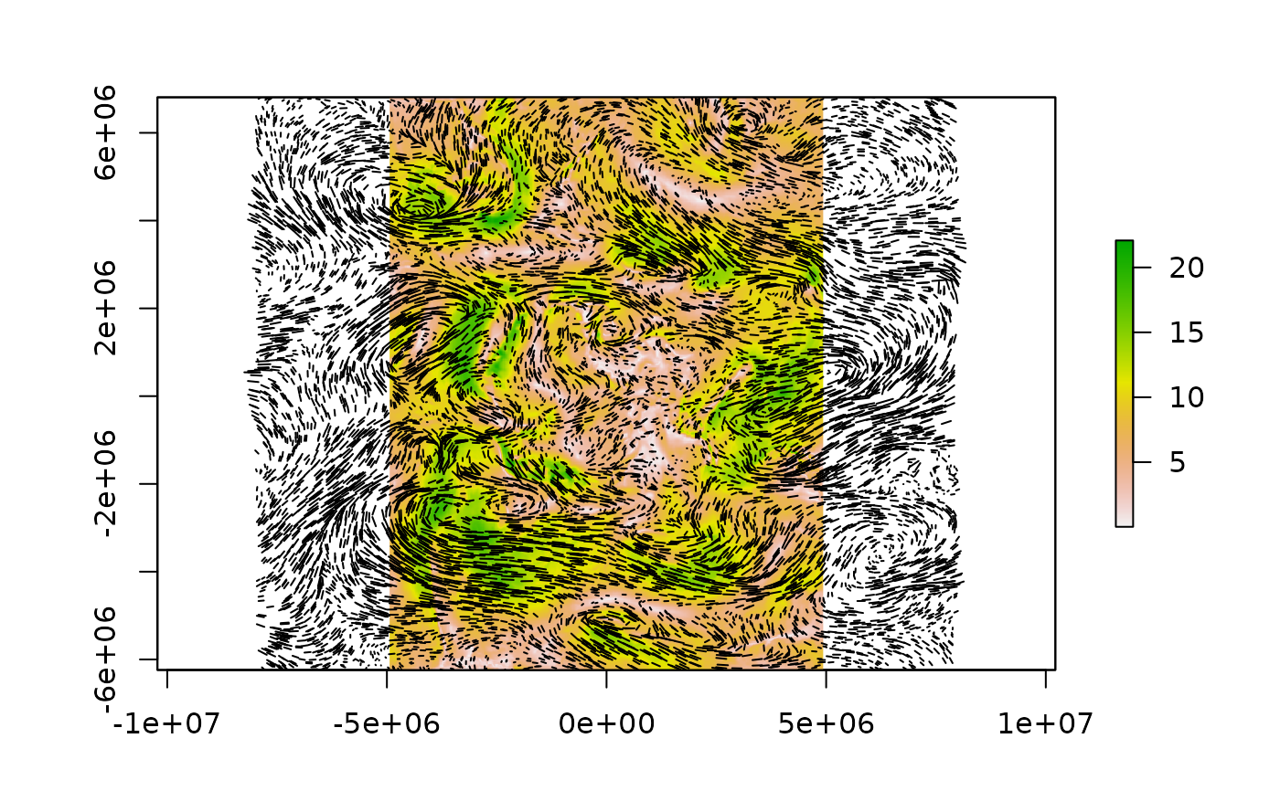
af <- amps_d1files()
w <- readamps_d1wind(latest = TRUE, inputfiles = af)
#w <- readamps_d2wind(latest = TRUE)
vlen <- function(a, b) sqrt(a * a + b * b)
plot(vlen(w[[1]], w[[2]]))

## arrow jigger
arr <- function(x, sub = seq(ncell(x[[1]])), scale = 1) {
 cr <- coordinates(x[[1]]); cr1 <- cr;
 cr1[,1] <- cr[,1] + values(x[[1]])*scale;
 cr1[,2] <- cr1[,2] + values(x[[2]]*scale);
 segments(cr[sub,1], cr[sub,2], cr1[sub,1], cr1[sub,2])
}
arr(w, sample(ncell(w), 10000), scale = 15000)
