Environmental data from an extent with raadtools
Michael Sumner and Jaimie Cleeland
2023-03-23
Source:vignettes/extract-extent.Rmd
extract-extent.RmdThe raadtools package contains a number of
read[something] functions, mostly for gridded time-series
remote sensing data.
All of the read functions have an “xylim” argument, which will take a
raster::extent(xmin, xmax, ymin, ymax). E.g.
## Loading required package: raster## Loading required package: sp## global option 'raadfiles.data.roots' set:
## '/rdsi/PRIVATE/raad/data
## /rdsi/PRIVATE/raad/data_local
## /rdsi/PRIVATE/raad/data_staging
## /rdsi/PRIVATE/raad/data_deprecated
## /rdsi/PUBLIC/raad/data '## Uploading raad file cache as at 2023-03-23 14:49:27 (1205841 files listed)## class : RasterLayer
## dimensions : 40, 240, 9600 (nrow, ncol, ncell)
## resolution : 0.25, 0.25 (x, y)
## extent : 100, 160, -50, -40 (xmin, xmax, ymin, ymax)
## crs : +proj=longlat +datum=WGS84 +no_defs
## source : memory
## names : Daily.sea.surface.temperature
## values : 4.41, 19.24 (min, max)
## time : 2010-01-01That extent must make sense for the data set though, so see what this returns first (it will be a longlat-grid in [-180, 180, -90, 90].
Note that we ran the function above without saving the result anywhere, so we just saw a print-out summary of the result but it is now discarded.
That is a useful technique to see what a function does, since it will return a layer by default. This can be plotted or used by other functions, and so is the best way to learn about the data source.
## class      : RasterLayer
## dimensions : 720, 1440, 1036800  (nrow, ncol, ncell)
## resolution : 0.25, 0.25  (x, y)
## extent     : -180, 180, -90, 90  (xmin, xmax, ymin, ymax)
## crs        : +proj=longlat +datum=WGS84 +no_defs
## source     : memory
## names      : Daily.sea.surface.temperature
## values     : -1.8, 32.61  (min, max)
## time       : 2023-01-31
That works for readssh, readcurr, and
readwind just the same, and the date argument can be a
single date or a vector of them. In the raster package
there are single RasterLayer objects and multi-layer
RasterBrick (or RasterStack) objects.
Raadtools will usually return a RasterStack or a RasterLayer, and it
will record the time-step/s on the data as well (when relevant). After
the read function is finished we are back to using the
raster package, so familiarity with that package and its
documentation is important.
vignette("Raster", package= "raster")Some of the functions respect lon180 = FALSE because
they have a grid that was originally in [0, 360, -90, 90]
and in that case it can be faster to use that domain for the extent
rather than the common [-180, 180, -90, 90] one. (Please
feel free to ask about this for specific data sets, it’s one of those
boring details).
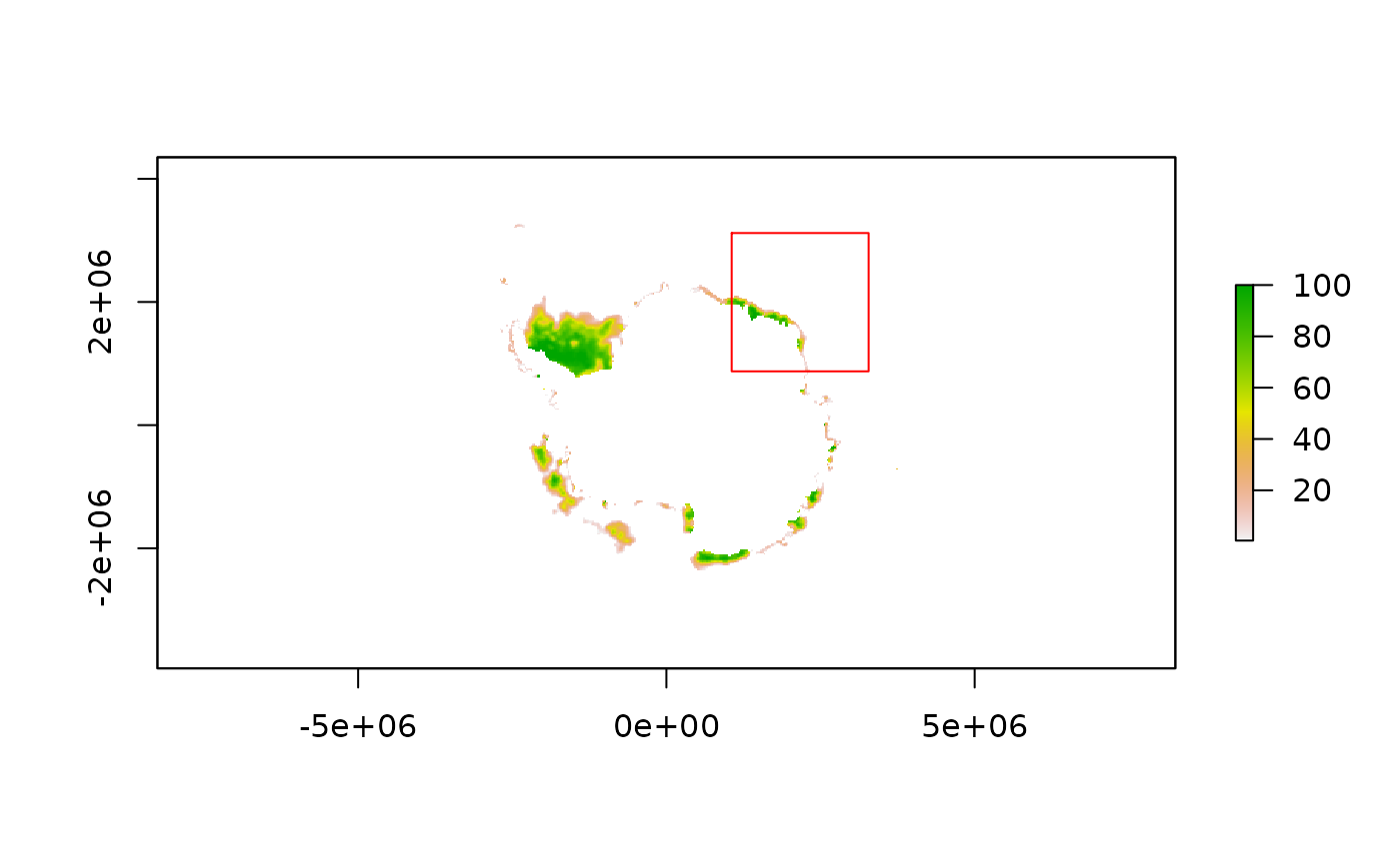
For ice, and some other data, the grids are not in longlat so
xylim needs an extent in that projection. You can always
draw one like this, with code that must be run interactively as the plot
will wait for you to click twice on the plot (defining a rectangle)
before the e object is created.
ice <- readice()
plot(ice)
e <- drawExtent()
Notice that we can also make
 Extent objects from scratch,
and perform operations on them.
my_extent <- extent(100, 120, -40, -20)
my_extent
## class : Extent
## xmin : 100
## xmax : 120
## ymin : -40
## ymax : -20
my_extent + 10## class : Extent
## xmin : 95
## xmax : 125
## ymin : -45
## ymax : -15otherwise there are functions projectExtent and some
others to do it more automatically. It’s not that straightforward
because of the polar aspect.
library(raadtools)
library(raadfiles)
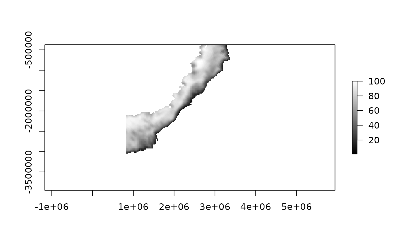
ice <- readice()
rex <- raster( extent(100, 160, -70, -50), crs = "+proj=longlat +datum=WGS84")
pex <- projectExtent(rex, projection(ice))
res(pex) <- 25000

ice_ex <- readice("2016-09-01", xylim = pex)

plot(ice_ex, col = grey(seq(0, 1, length = 100)), zlim = c(1, 100))
Please note that the xylim argument just applies
crop, so you can avoid it altogether and do it after the
fact.
## class      : RasterLayer
## dimensions : 40, 240, 9600  (nrow, ncol, ncell)
## resolution : 0.25, 0.25  (x, y)
## extent     : 100, 160, -50, -40  (xmin, xmax, ymin, ymax)
## crs        : +proj=longlat +datum=WGS84 +no_defs
## source     : memory
## names      : Daily.sea.surface.temperature
## values     : 4.49, 21.96  (min, max)
## time       : 2023-01-31
(Internally raadtools always uses snap=out
since that makes sure the intersection is inclusive, i.e. any
overlapping part of a pixel means that pixel is included in the result.
By default crop would drop partial overlaps on the
edge).
If there’s a really long time series though it will be better to do that with xylim, and even to pass it out to a file:
More details … TBD
Extending maps
With two examples from above.
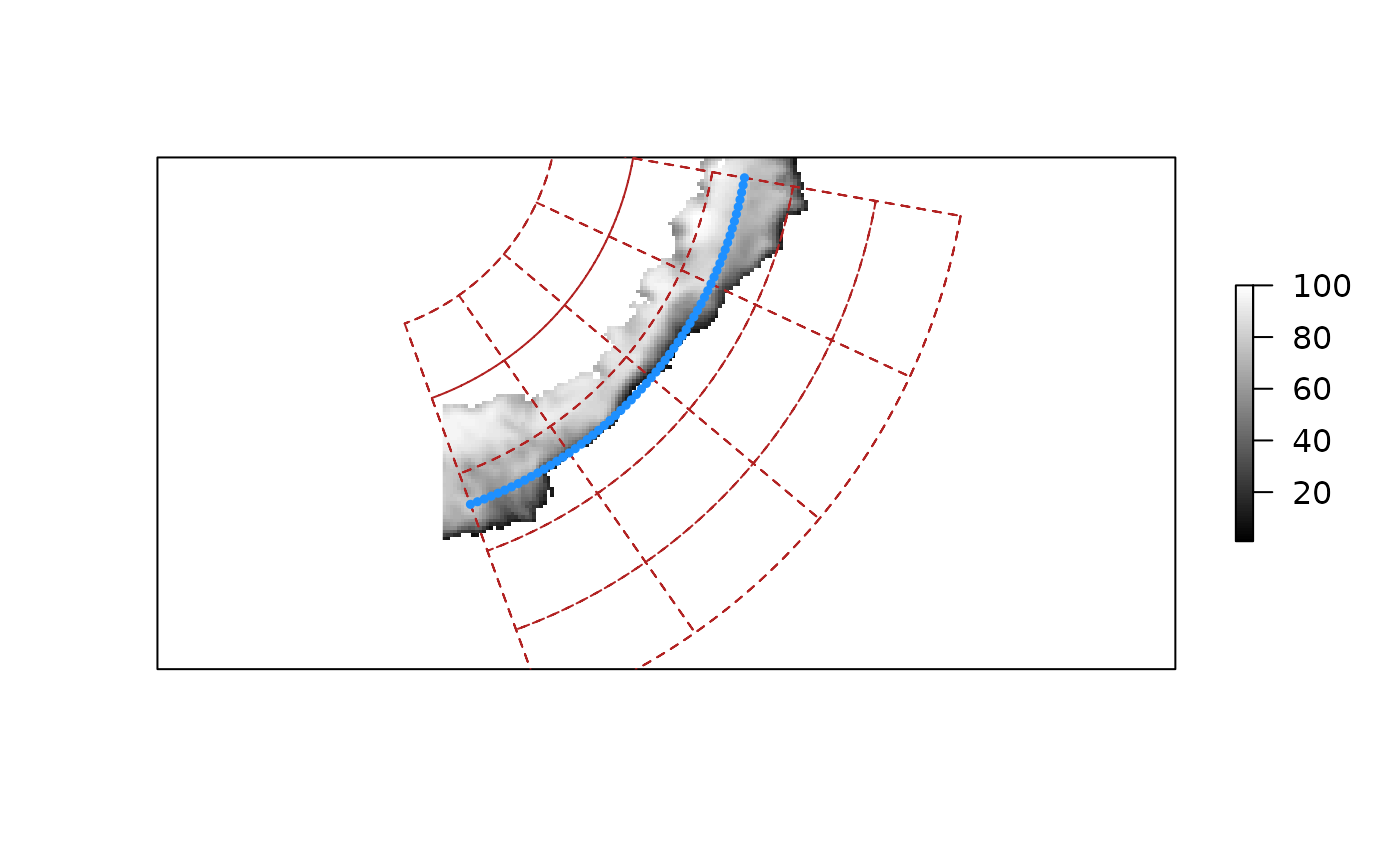
Plot the projected data with a graticule, and add a “transect”.
library(raadtools)
library(raadfiles)
ice <- readice()
rex <- raster( extent(100, 160, -70, -50), crs = "+proj=longlat +datum=WGS84")
pex <- projectExtent(rex, projection(ice))
res(pex) <- 25000

ice_ex <- readice("2016-09-01", xylim = pex)

## create a graticule for this region

g <- graticule::graticule(seq(100, 160, by = 15), seq(-75, -50, by = 5), proj = projection(ice))
plot(ice_ex, col = grey(seq(0, 1, length = 100)), zlim = c(1, 100), axes = FALSE,
     addfun = function() plot(g, add = TRUE, lty = 2, col = "firebrick"))

## add a "transect"
lons <- seq(100, 160, by = 1)
transect <- rgdal::project(cbind(lons, -63), projection(ice_ex))
## Warning: PROJ support is provided by the sf and terra packages among others
points(transect, cex = 0.5, pch = 19, col = "dodgerblue")
Extract values at specific points.
library(raadtools)
library(raadfiles)
iceconc <- extract(ice_ex, transect, method = "bilinear")
plot(lons, iceconc, main = "ice concentration at latitude -65 between 100E and 160E")
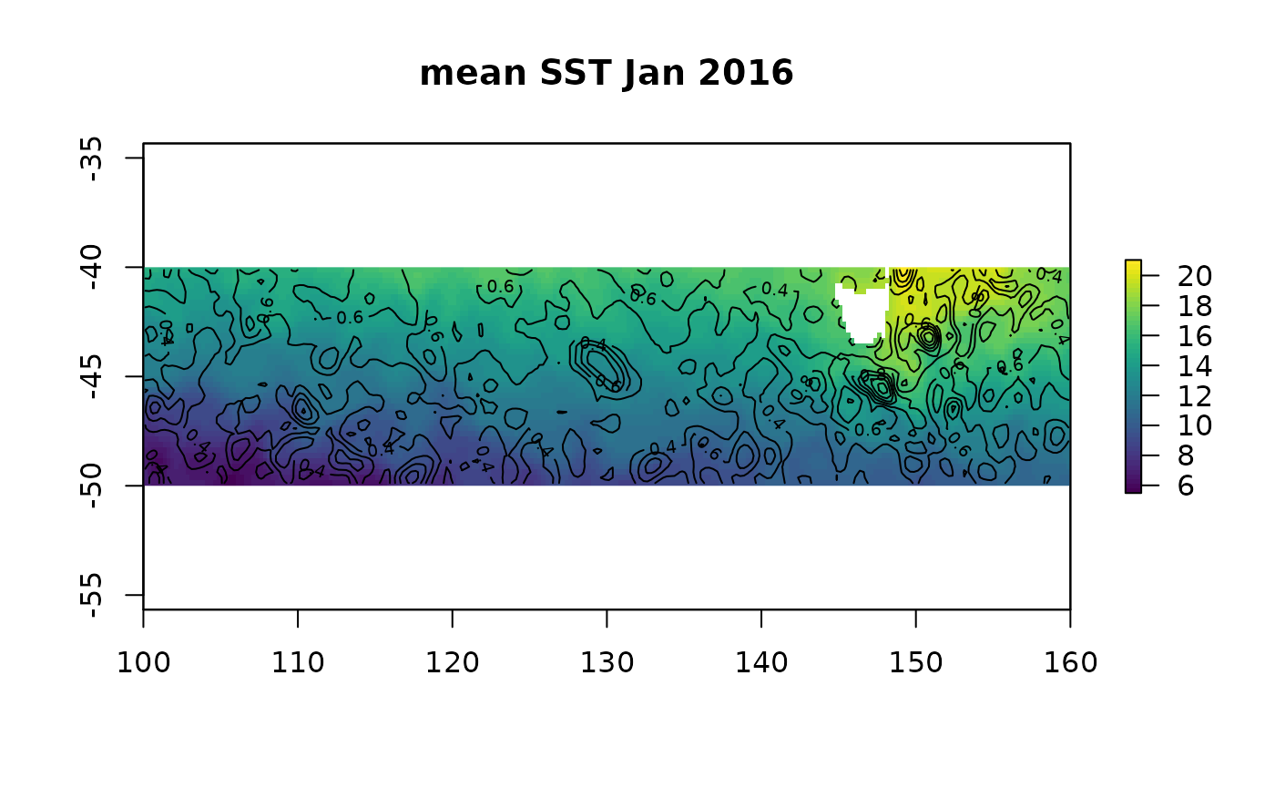
Plot mean SST and contour.
library(raadtools)
library(raadfiles)
dates <- seq(as.Date("2016-01-01"), length = 31, by = "1 day")
sst <- readsst(dates,  xylim = extent(100, 160, -50, -40))
msst <- calc(sst, mean)
sdsst <- calc(sst, sd)
plot(msst, col = viridis::viridis(50), main = "mean SST Jan 2016",  addfun = function() contour(sdsst, add = TRUE))