Southern Ocean Fronts for R
Michael Sumner
2022-10-10
Source:vignettes/orsifronts.Rmd
orsifronts.RmdOrsi fronts for R
The “Orsi fronts” are a commonly used climatological map of Southern Ocean frontal distributions, once published on a Southern Ocean Atlas Database Page after Orsi et al. (1995).
The data is provided in this package as a built-in data set. The object orsifronts is a ‘SpatialLinesDataFrame’ object, as defined in the ‘sp’ package. (A ‘SpatialLinesDataFrame’ is a “GIS vector” layer where complex line geometry objects are linked to simple attribute data in a table form, and it behaves like a ‘data.frame’).
library(orsifronts)
#> Loading required package: sp
cols <- hcl(seq(0, 240, length = nrow(orsifronts)), c = 50)
plot(orsifronts, col = cols, lwd = 2)
degAxis(1)
degAxis(2)
box()
There are 5 line objects, with some simple names and codes.
as.data.frame(orsifronts)
#>                                                         name front
#> stf                                        Subtropical front   stf
#> saf                                       Subantarctic front   saf
#> pf                                               Polar front    pf
#> saccf           Southern Antarctic circumpolar current front saccf
#> sbdy  Southern Boundary of the Antarctic circumpolar current  sbdy
plot(orsifronts, xlim = c(60, 180), col = cols, asp = 1/cos(55 * pi / 180), lwd = 4)
legend("topleft", sprintf("%s (%s)", orsifronts$front, orsifronts$name),
       col = cols, lwd = 4, cex = 0.8, bty = "n")
degAxis(1)
degAxis(2)
box()
Park/Durand fronts for R
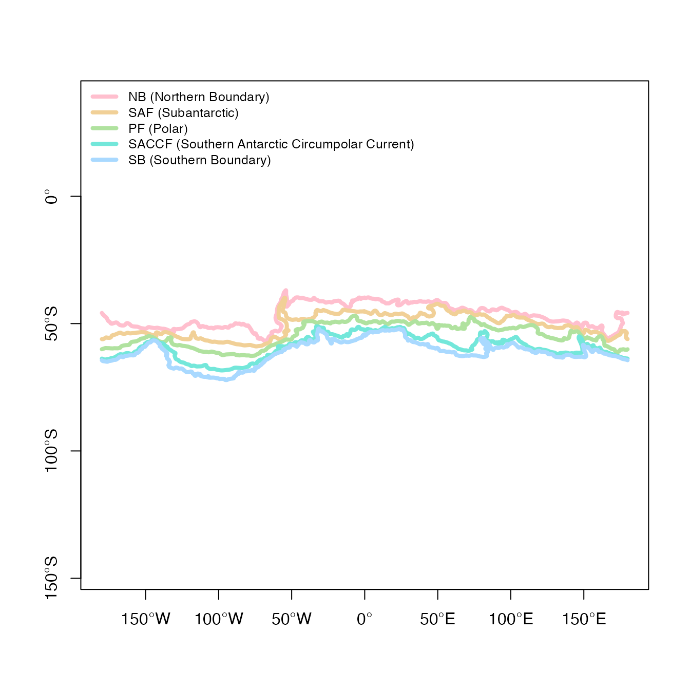
Similarly for the more recent Park/Durand fronts derived from altimetry remote sensing.
as.data.frame(parkfronts)
#>                                     name front
#> 1                      Northern Boundary    NB
#> 2                           Subantarctic   SAF
#> 3                                  Polar    PF
#> 4 Southern Antarctic Circumpolar Current SACCF
#> 5                      Southern Boundary    SB
pcols <- hcl(seq(0, 240, length = nrow(parkfronts)), c = 50)
plot(parkfronts,col = pcols, asp = 1/cos(55 * pi / 180), lwd = 4)
legend("topleft", sprintf("%s (%s)", parkfronts$front, parkfronts$name),
       col = cols, lwd = 4, cex = 0.8, bty = "n")
degAxis(1)
degAxis(2)
box()