library(aceecostats)
library(sp)

knitr::kable(as.data.frame(aes_zone))

SectorName	Zone	area_km2	colour	ID
Atlantic	High-Latitude	19855197.0	#7CAE0099	1
Atlantic	Continent	1084548.0	#7CAE00FF	2
Atlantic	Mid-Latitude	15671351.4	#7CAE004D	3
EastPacific	High-Latitude	3241353.4	#C77CFF99	4
EastPacific	Continent	724857.5	#C77CFFFF	5
EastPacific	Mid-Latitude	10573933.0	#C77CFF4D	6
Indian	High-Latitude	11699156.9	#00BFC499	7
Indian	Continent	706453.8	#00BFC4FF	8
Indian	Mid-Latitude	13068371.7	#00BFC44D	9
WestPacific	High-Latitude	8136176.3	#F8766D99	10
WestPacific	Continent	885409.0	#F8766DFF	11
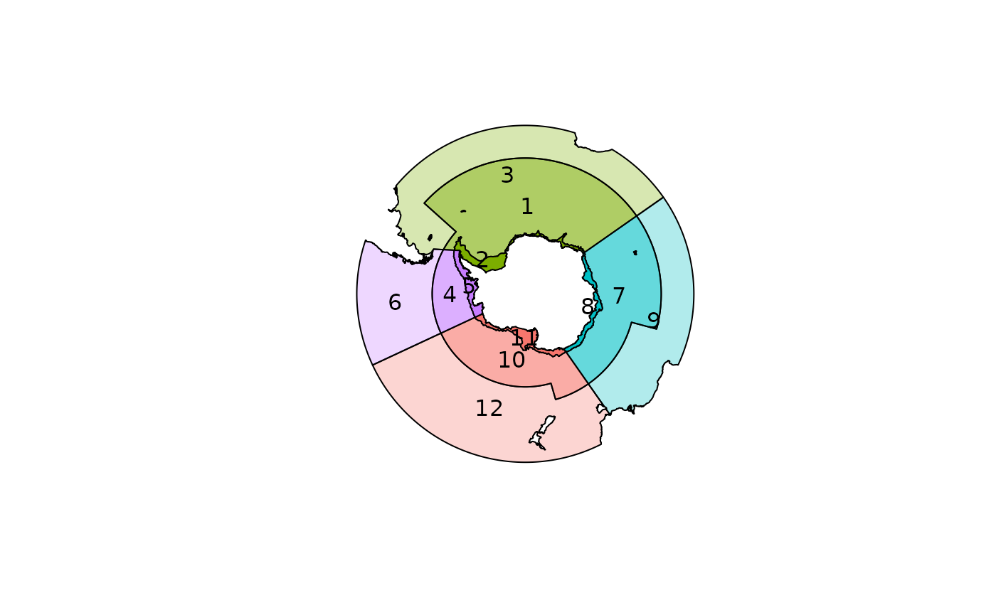
WestPacific	Mid-Latitude	23025500.3	#F8766D4D	12

Area

There are 12 regions classified by SectorName, and Zone.

plot(aes_zone, col = aes_zone$colour)
text(coordinates(aes_zone), lab = aes_zone$ID)