Processing Workflow

This is in-progress, current map of the entire process is here: https://github.com/AustralianAntarcticDivision/aceecostats/issues/14

Install

Install the package

devtools::install_github("AustralianAntarcticDivision/aceecostats")

Regions

Get the regions.

library(aceecostats)
library(sp)
labs <- data.frame(x= c(112406,4488211,-1734264,-4785284), y=c(4271428,-224812,-3958297,-104377), labels=c("Atlantic","Indian", "West Pacific", "East Pacific"))
labs <- SpatialPointsDataFrame(labs[,1:2],labs, proj4string = CRS(proj4string(aes_zone)))
plot(aes_zone, col = aes_zone$colour, border="grey")
text(labs$x, labs$y, labs$labels, cex=0.6)

# latitude zone labels
lat.labs<- function(the.proj="polar"){
  if(the.proj=="latlon"){
    ext <- extent(aes_zone_ll)
    text("Polar", x=ext@xmin, y=ext@ymin, xpd=NA, pos=2, cex=0.6)
    text("High latitude", x=ext@xmin, y=ext@ymin*0.8, xpd=NA, pos=2, cex=0.6)
    text("Mid latitude", x=ext@xmin, y=ext@ymin*0.6, xpd=NA, pos=2, cex=0.6)
  }
  if(the.proj=="polar"){
    text(c("Polar", "High latitude", "Mid latitude"), x=c(113064.6,-1017581.1,-3642294), y=c(-1518296,-2285519,-3012363), cex=0.5, col=rgb(0,0,0,0.7))
  }
}
lat.labs()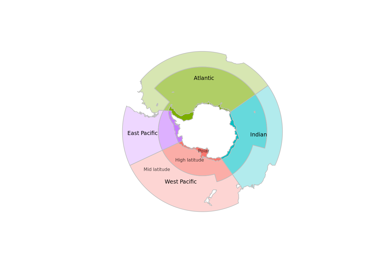

In unprojected form.

library(aceecostats)
library(raster)
library(sp)
plot(aes_zone_ll, col = aes_zone_ll$colour, border="grey")
ll_labs <- spTransform(labs, CRS(proj4string(aes_zone_ll)))
text(ll_labs$x, ll_labs$y, labels=labs$labels, cex=0.6)
lat.labs("latlon")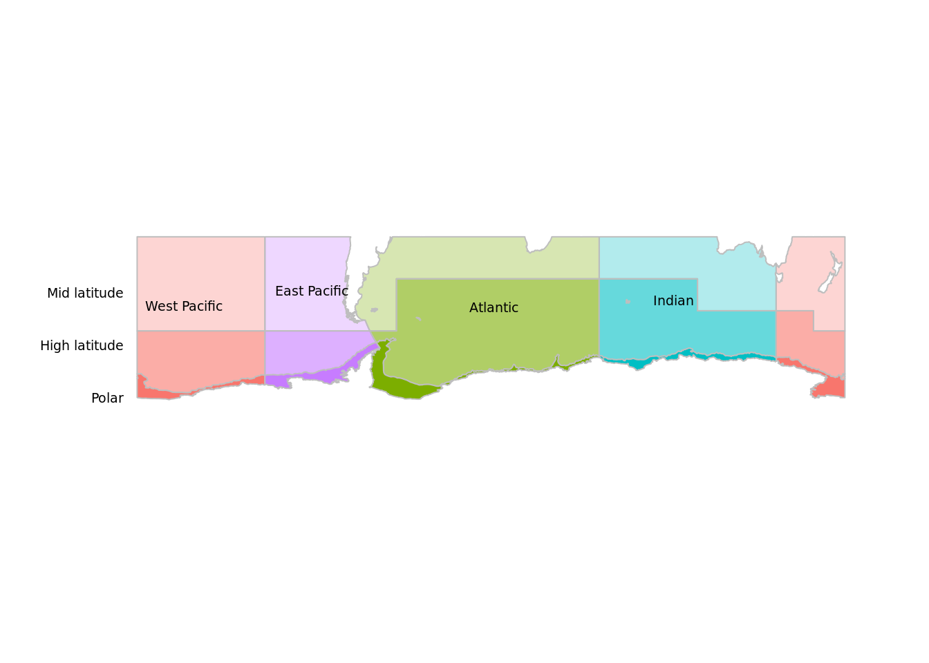

Metadata

The data is stored on the map object itself.

knitr::kable(as.data.frame(aes_zone))

SectorName	Zone	area_km2	colour	ID
Atlantic	High-Latitude	19855197.0	#7CAE0099	1
Atlantic	Continent	1084548.0	#7CAE00FF	2
Atlantic	Mid-Latitude	15671351.4	#7CAE004D	3
EastPacific	High-Latitude	3241353.4	#C77CFF99	4
EastPacific	Continent	724857.5	#C77CFFFF	5
EastPacific	Mid-Latitude	10573933.0	#C77CFF4D	6
Indian	High-Latitude	11699156.9	#00BFC499	7
Indian	Continent	706453.8	#00BFC4FF	8
Indian	Mid-Latitude	13068371.7	#00BFC44D	9
WestPacific	High-Latitude	8136176.3	#F8766D99	10
WestPacific	Continent	885409.0	#F8766DFF	11
WestPacific	Mid-Latitude	23025500.3	#F8766D4D	12

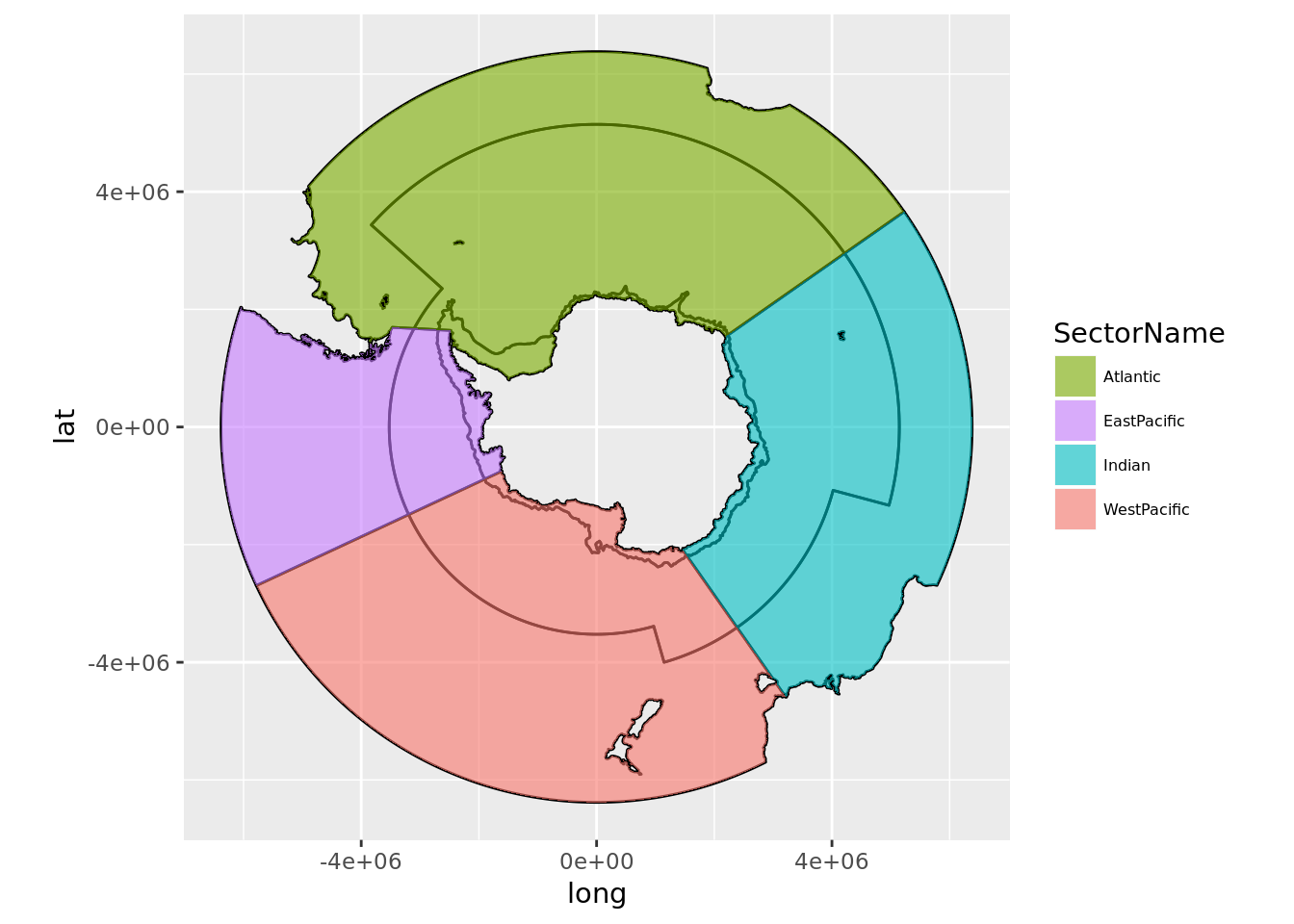
Prefer ggplot2?

## TODO fix this code
library(ggplot2)
library(ggpolypath)
tab <- fortify(aes_zone)

## Regions defined for each Polygons

zcols <- as.data.frame(aes_zone)[, c("colour", "SectorName", "Zone")]
tab$SectorName <- zcols$SectorName[factor(tab$id)]
ggplot(tab) + aes(x = long, y = lat, group = group, fill = SectorName) + scale_fill_manual(values = setNames(zcols$colour, zcols$SectorName)) + geom_path() + 
geom_polypath() + theme(legend.text=element_text(size=6)) + guides(position = "bottom") + coord_equal()