Compare two different estimations of biomass movement

This function compares - graphically and analytically - two estimations of biomass movement over the same domain, which will usually be the results of two different algorithms.

biomass.compare(N1, N2, graphics = TRUE, legend = NULL)

Arguments

N1

An object of class biomass\_distribution.

N2

An object of class biomass\_distribution.

graphics

If TRUE, the times series' for the different polygons are plotted.

legend

If one of the legend-location keywords (see ?legend) or a location (see ?locator) is given, a legend is drawn at the requested location. If NULL, no legend is drawn.

Value

Two distance measures of the two time series, namely the average squared difference between two corresponding entries in the matrices N1 and N2 and the average relative deviation,

sum((N1-N2)^2)/n

and

sum(abs(N1-N2)/(N1+N2)/n

Details

The objects N1 and N2 both contain information about the time points at which they were calculated, to ensure both are comparable. In the rest of this document, N1 and N2 refer to the time series only, which are really N1$bmdist and N2$bmdist.

It is assumed that N1 and N2 describe biomass distributions over the same time intervals and over the same domain, as there is no way for the function to check this. N1 and N2 have to be matrices of dimension 'number of polygons' x 'number of time steps'.

Author

Thorsten Lenser

Examples

## Generate two sample time series with two polygons
N1 = (seq(0,98,length=50)/10)^2
N1 = matrix(c(N1,N1[50:1]), nrow=2, byrow=TRUE)
N2 = N1[1,] + rnorm(50,sd=3)
N2 = matrix(c(N2,N2[50:1]), nrow=2, byrow=TRUE)

## Turn into objects of class "biomass_distribution"
N1 = list(bmdist=N1,times=seq(0,98,length=50))
N2 = list(bmdist=N2,times=seq(0,98,length=50))
class(N1) = "biomass_distribution"
class(N2) = "biomass_distribution"

## Compare them
biomass.compare(N1,N2)

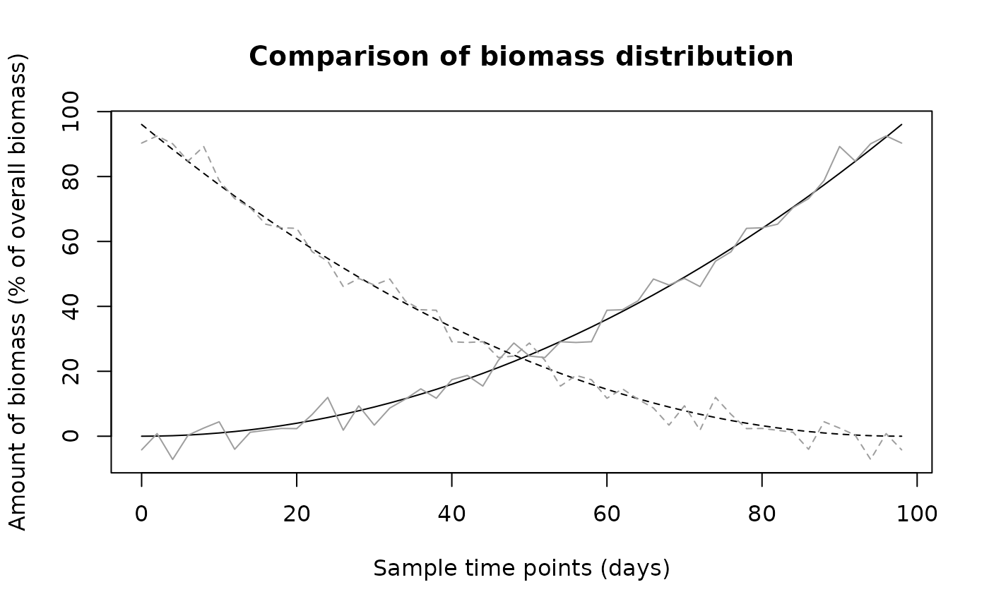#> [1] 20.46445515  0.06146867