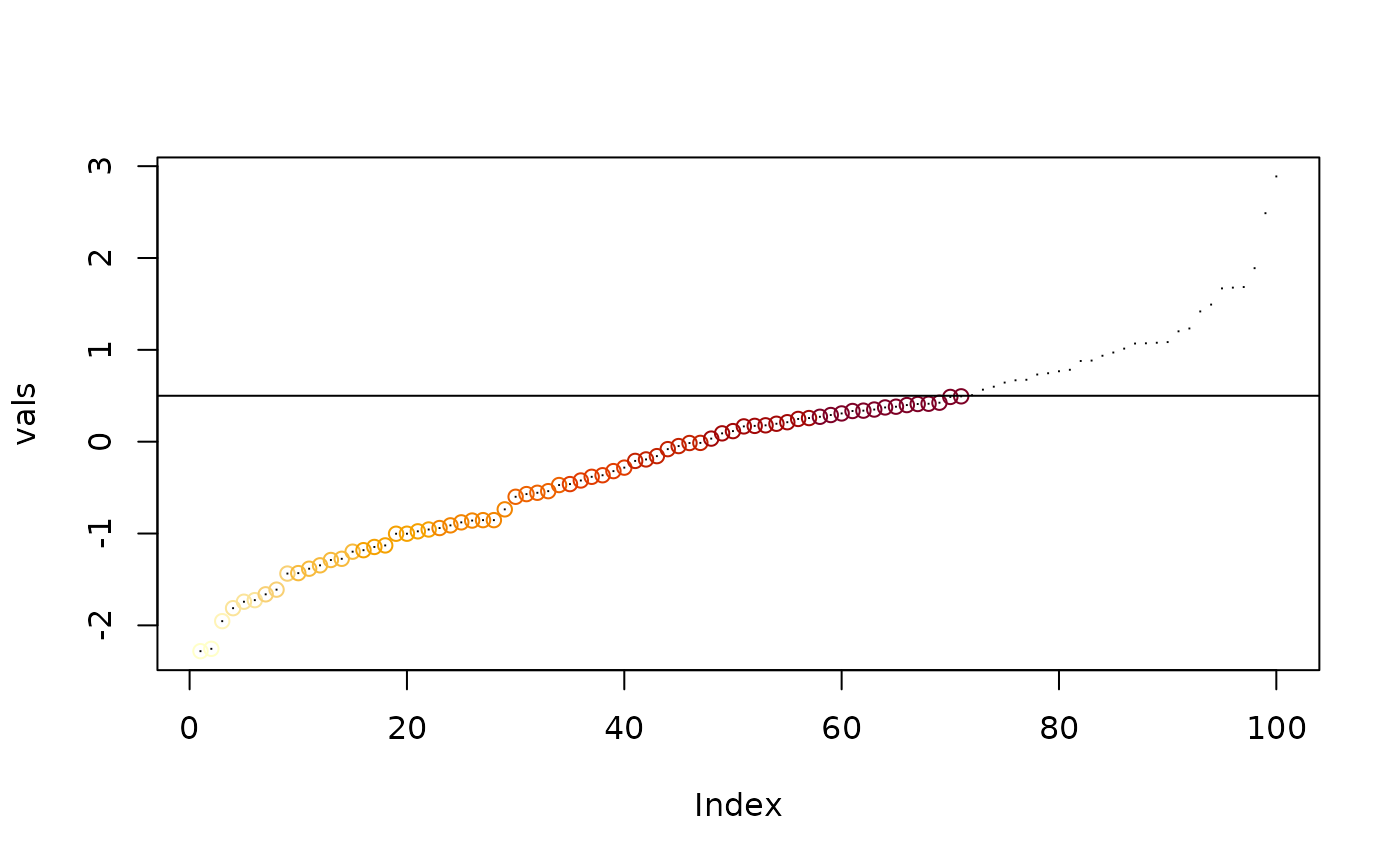
If no `col` is provided, the default image palette is used. The density can be controlled with `n` and the mapping with the optional `breaks`. If `breaks` is included as well as `n`, `n` is ignored.
image_pal(x, col, ..., breaks = NULL, n = NULL, zlim = NULL)

image_raster(x, col, ..., breaks = NULL, n = NULL, zlim = NULL)

image_stars(x, col, ..., breaks = NULL, n = NULL, zlim = NULL)
Arguments
- x
numeric values, raster object (single layer only) or stars object (single variable, 2D array only)
- col
function to generate colours, or a vector of hex colours
- ...
ignored
- breaks
optionally used to specify colour mapping
- n
optionally used to specify density of colours from `col` (ignored if `breaks` is set)
- zlim
numeric range to clamp values to an absolute scale (ignored if `breaks` is set)
Value
for `image_pal()` a vector of hex colours, for `image_raster` and `image_stars` a raster or stars object with 3 channel RGB (range 0,255)
Details
The function `image_pal()` only returns hex character string colours. The function `image_raster()` will map a raster of numeric values to an RGB 3-layer (channel) raster brick, and `image_stars()` similarly for a 3-dimensional stars object.
Please note that the expansion to 3-channels is a fairly wasteful thing to do, the overall data is expanded from a single layer to three but this faciliates a specific task of creating textures for 3D mapping, and this is the only way to do it currently. It's also useful in other situations, for controlling exactly the kind of plots we can achieve and for exporting to image formats such as 'GeoTIFF' or 'PNG'.
